Executive Summary: Bridging Mathematical Network Solvers with C-Suite Capital Allocation
Supply chain network optimization studies represent some of the highest-stakes capital and operational decisions an enterprise will ever execute. Reconfiguring a global or continental supply chain—opening advanced automated distribution centers (DCs), rationalizing legacy manufacturing plants, nearshoring production hubs, renegotiating multi-modal freight lanes, and reallocating regional customer territories—routinely demands between $50 million and $300 million in cumulative capital expenditures (CapEx) and transition OpEx. Yet, over 65% of supply chain network design proposals stall, face prolonged executive committee scrutiny, or suffer fatal scope dilution during boardroom reviews.
The root cause of this failure is rarely analytical flaw in the underlying mathematical optimization engine. Modern supply chain design teams leverage sophisticated mixed-integer linear programming (MILP) tools, center-of-gravity solvers, and digital twins (such as Coupa/Llamasoft Supply Chain Guru, AnyLogistix, or Blue Yonder) that evaluate hundreds of thousands of candidate lane assignments and discrete facility variables. Instead, the failure is almost exclusively presentational: supply chain leaders arrive at the Executive Committee or Board of Directors with 80-slide decks filled with raw solver logs, unreadable spaghetti GIS maps showing tens of thousands of individual freight lanes, and academic sensitivity tables formatted in 8-point font.
To senior executives—specifically the Chief Executive Officer (CEO), Chief Financial Officer (CFO), and Board Investment Committee—an optimization deck must not look like an operations research doctoral thesis. It must function as a strategic capital allocation and risk mitigation memorandum. C-suite decision-makers do not evaluate individual pallet handling tariffs or mile-by-mile diesel surcharge curves; they evaluate four macro dimensions:
1. Strategic Resilience & Market Agility: Does this network topology reduce lead times to core growth markets, hedge against geopolitical or tariff disruptions, and protect customer On-Time In-Full (OTIF) delivery during regional black-swan shocks? 2. Financial Return & Payback Velocity: What is the audited Net Present Value (NPV), Internal Rate of Return (IRR), and discounted payback period across multi-year CapEx tranches, and how quickly does the business achieve sustainable operating margin expansion? 3. Total Cost-to-Serve (TCS) Dynamics: How does the proposed configuration resolve the fundamental structural trade-off between inbound transportation, manufacturing conversion costs, fixed facility overhead, and outbound last-mile parcel/LTL fulfillment? 4. Transition Risk & Operational Continuity: What is the phased cutover sequence, how are customer service-level agreements (SLAs) safeguarded during inventory rebalancing, and what are the explicit stage-gate go/no-go milestones?
This guide outlines the end-to-end framework for architecting an institutional-grade supply chain network optimization presentation. Drawing on best practices from top-tier operations management consultancies (McKinsey Operations, Kearney, Bain, and BCG) and leading multinational supply chain organizations, we provide the exact narrative sequencing, quantitative slide layouts, cost waterfalls, site selection matrices, and prompt recipes necessary to secure unanimous board approval for complex network transformations.
The 5 Core Supply Chain Network Optimization Presentation Archetypes
Supply chain presentations vary dramatically depending on corporate context, deal catalysts, and capital constraints. Selecting the correct presentation archetype ensures your deck aligns with executive expectations.
| Deck Archetype | Primary Catalyst & Trigger | Target Decision-Making Audience | Core Analytical Focal Point | Decisive Board Deliverable / Outcome |
|---|---|---|---|---|
| Continental Distribution Center (DC) Rationalization | Post-merger overlapping network or legacy multi-node DC sprawl causing excessive inventory carrying costs and poor SLA performance | Chief Operating Officer (COO), Chief Commercial Officer (CCO), and Chief Financial Officer (CFO) | Center-of-gravity demand modeling, outbound LTL/parcel transit time bands, and warehouse automation throughput economics | Consolidation of 14 regional warehouses into 4 mega-automated omni-channel hubs with audited $28M annual operating expense savings |
| Manufacturing Footprint & Nearshoring Restructuring | Rising offshore labor rates, maritime freight volatility, tariff barriers (Section 301/USMCA), and extended supply lead times | Board of Directors, CEO, and Executive Strategy & Capital Allocation Committee | Landed cost-to-serve parity analysis, regional labor availability/arbitrage, cross-border customs compliance, and plant retooling CapEx | Board authorization of a $120M brownfield assembly expansion in northern Mexico coupled with strategic capacity ramp in the US Southeast |
| Omnichannel & Direct-to-Consumer (DTC) Node Deployment | Shift from traditional pallet/case B2B retail distribution toward rapid next-day and same-day e-commerce consumer fulfillment | Chief Digital Officer (CDO), Chief Supply Chain Officer (CSCO), and VP of E-Commerce | Customer density radius mapping, last-mile parcel rate zone skipping, micro-fulfillment center (MFC) economics, and inventory pooling | Deployment of 6 regional forward stocking locations (FSLs) with integrated 3PL multi-tenant fulfillment enabling 94% next-day ground coverage |
| Supply Chain Decarbonization & ESG Network Redesign | Corporate net-zero carbon mandates, Scope 3 greenhouse gas reporting regulations (SEC/CSRD), and green logistics requirements | Board Sustainability Committee, Chief Risk Officer (CRO), and Institutional Investors | Ton-kilometer freight emissions modeling, modal shift optimization (over-the-road trucking to rail intermodal), and LEED DC certification | 18% reduction in network transportation carbon emissions while maintaining sub-48-hour delivery SLAs through electrified short-haul drayage |
| Private Equity 100-Day Supply Chain Value Creation | Post-acquisition portfolio company carve-out, gross margin expansion mandate, or preparation for EBITDA exit multiple arbitrage | PE Deal Sponsors, Operating Partners, Portfolio Company CEO, and Lender Syndicate | Rapid cost-to-serve benchmarking, working capital cash liberation via safety stock consolidation, and 3PL contract rebidding | Underwritten 180-basis-point gross margin expansion and $42M working capital release within 18 months of transaction close |
Exhibit 1: Manufacturing & Distribution Network Topology: Baseline vs. Nearshore vs. Regional Hubs (Scenario Comparison Matrix)
Key Supply Chain Network Optimization Takeaways for CSCOs, COOs & Operations Consultants
- Frame the Network as a Dynamic Economic Engine, Not a Fixed Asset Map: Executive committees do not approve geographic maps; they fund margin expansion, inventory reduction, and risk hedges. Every network proposal must explicitly tie facility topology to P&L gross margins, working capital velocity, and enterprise return on invested capital (ROIC).
- Lead with the Unconstrained Center-of-Gravity (COG) Baseline: Anchor your executive narrative by revealing where your network mathematically SHOULD be located based purely on weighted customer demand and supplier origins, before layering on real-world industrial real estate, labor pool, and highway infrastructure constraints.
- Decompose Delivered Cost-to-Serve into Discrete P&L Levers: Disaggregate complex supply chain expenditures into four interdependent pillars: Inbound Freight (ocean/rail/intermodal), Manufacturing Conversion Costs, Fixed Facility Overhead & Warehousing OpEx, and Outbound Transportation (FTL/LTL/Parcel). Prove to the CFO how savings in one bucket outweigh investments in another.
- Respect the Fundamental Inventory-Transportation Trade-Off: Adding distribution nodes reduces outbound transit times and parcel shipping costs, but exponentially fragments inventory across stocking locations, driving up safety stock under the Square Root Law. Present clear multi-scenario frontier curves that expose this trade-off.
- Structure Site Selection Around a 100-Point Weighted Due Diligence Scorecard: Eliminate regional bias and emotional executive preferences by evaluating candidate cities across audited metrics: 24-hour truck drive-time radius, industrial warehouse lease rates per square foot, prevailing warehouse labor wage rates, state corporate tax incentives, and utility power grid reliability.
- Enforce Stage-Gate Capital Governance Across a 24-Month Phased Migration: Mitigate executive fear of customer fulfillment disruptions by structuring network migration into sequential stage gates (Phase 1: Diagnostic & Blueprint; Phase 2: Pilot Facility Cutover; Phase 3: Core Regional Node Go-Live; Phase 4: Legacy Node Decommissioning & Real Estate Liquidation).
Center-of-Gravity (COG) Analytics & Baseline Network Diagnostics: Establishing the Unconstrained Demand Anchor
Every compelling supply chain network optimization narrative begins with rigorous diagnostic grounding. Senior executives and board members frequently harbor historical biases regarding why specific plants or warehouses exist in their current locations. Often, an enterprise's physical footprint is the accidental byproduct of decades of unintegrated bolt-on acquisitions, long-expired state tax abatements, or legacy proximity to the original founder's hometown. To disarm institutional inertia, the presenter must establish an objective mathematical benchmark: the unconstrained Center-of-Gravity (COG) baseline.
### The Mathematical Center-of-Gravity Formulation The center-of-gravity calculation identifies the theoretical optimal coordinate point $(X^*, Y^*)$ on a geographic plane that minimizes total transportation ton-mile costs. By weighting each customer shipping destination $i$ and supplier origin point $j$ by annual volume (in hundredweight [CWT] or metric tons) and specific transportation cost rates ($C_i$), the solver calculates the weighted centroid:
$X^* = \frac{\sum (X_i \cdot W_i \cdot C_i)}{\sum (W_i \cdot C_i)}, \quad Y^* = \frac{\sum (Y_i \cdot W_i \cdot C_i)}{\sum (W_i \cdot C_i)}$
When presenting this slide to the C-suite, follow the 'Current Reality vs. Mathematical Ideal' visual contrast. Display a clean, dual-panel executive map: - Left Panel (The Inherited Baseline): Depict the current operational network (e.g., 18 fragmented warehouses). Annotate the severe operational friction points: cross-shipping between overlapping regional territories (where a facility in Memphis ships goods to an account in Ohio while a warehouse in Pennsylvania ships identical SKUs to Kentucky), average outbound transit distance (e.g., 685 miles), and customer volume captured within 1-day ground transit (e.g., only 48%). - Right Panel (The Unconstrained 4-Node Centroid): Display the pure mathematical centroids generated by the MILP solver based on 3-year forward demand projections. Show how clustering demand around 4 optimized regional epicenters (e.g., Allentown PA for the Northeast, Atlanta GA for the Southeast, Dallas-Fort Worth for South Central, and Inland Empire/Reno for the West Coast) immediately slashes average outbound haul distance from 685 miles down to 240 miles.
### Diagnostic Baseline Metrics Table Accompany the geographic visual with a clean, 4-row executive diagnostic table that establishes the economic baseline against which all future optimization scenarios will be measured: 1. Total Annual Delivered Volume: Annual tonnage shipped (e.g., 450,000 tons / 18.2 million units) and total annual freight spend ($142.5 million). 2. Service Level Delivery Velocity: Current percentage of customer demand reached within 1-day ground (48.2%), 2-day ground (81.4%), and 3+ days (18.4%). 3. Fleet & Lane Utilization Efficiency: Percentage of outbound volume shipped Full Truckload (FTL - 42%) vs. Less-Than-Truckload (LTL - 38%) vs. Expedited Parcel (20%), highlighting excessive freight mode premiums. 4. Network Cost-to-Serve Baseline: Current total delivered cost per unit ($7.83/unit) broken down by manufacturing conversion ($3.15), inbound transportation ($0.88), warehousing and handling ($1.65), outbound linehaul/LTL ($1.85), and inventory carrying cost ($0.30).
By establishing this unassailable quantitative baseline, the presenter shifts the conversation from subjective opinions ('We have always had a warehouse in Indianapolis') to undeniable economic facts ('Our current Indianapolis facility sits 210 miles away from our modern customer demand weighted center, adding $4.2M in redundant annual linehaul costs').
Exhibit 2: Total Logistics Cost-to-Serve Optimization: Inbound Freight, Plant Conversion, Warehousing, and Outbound Last-Mile Savings Waterfall
Decomposing Total Landed Cost-to-Serve: Inbound Freight, Manufacturing Conversion, Fixed Facilities & Last-Mile Transportation
The single most common error in supply chain presentations is presenting freight savings in isolation. An operations team might proudly present a warehouse consolidation plan that slashes real estate lease costs by $15 million, only for an astute CFO to point out that the consolidated network increases outbound customer shipping distances, triggering $22 million in additional LTL freight expenses—resulting in a net $7 million P&L loss. To earn executive credibility, your presentation must anchor on Total Landed Cost-to-Serve (TCS).
### The 4 Pillars of Delivered Cost-to-Serve A rigorous network optimization presentation decomposes delivered cost into four interdependent operational buckets:
1. Inbound Sourcing & Primary Linehaul ($/CWT or $/Unit): - Evaluates the cost of transporting raw materials and finished goods from tier-1 suppliers, contract manufacturing partners, and maritime ocean ports to primary production plants or regional import deconsolidation centers. - Key variables include container drayage rates, port congestion demurrage, rail intermodal vs. long-haul trucking rates, and volume-tiered freight contracts. - Trade-off dynamics: Concentrating manufacturing or assembly in a single mega-plant maximizes inbound supplier purchasing scale and simplifies raw material delivery, but forces longer domestic linehaul routes to regional distribution points.
2. Manufacturing & Assembly Conversion Costs ($/Unit): - Measures direct labor, machine depreciation, facility utility overhead, and plant scrap/yield rates across regional manufacturing locations. - Evaluates wage differentials (e.g., $28.50/hour union manufacturing labor in the US Midwest vs. $6.20/hour fully burdened labor in Monterrey, Mexico). - Trade-off dynamics: Highly automated, centralized manufacturing achieves massive economies of scale and low unit conversion costs, but creates single-point-of-failure vulnerabilities and multi-week transit pipelines.
3. Warehousing, Facility Leases & Material Handling OpEx ($/Sq Ft & $/Pallet Move): - Encompasses industrial real estate triple-net (NNN) lease rates, warehouse management system (WMS) licensing, material handling equipment (MHE) amortization (e.g., autonomous mobile robots [AMRs], automated storage and retrieval systems [ASRS]), and warehouse labor. - Trade-off dynamics: Operating 15 regional warehouses requires 15 distinct building leases, 15 local supervisory teams, and duplicated handling equipment. Consolidating into 4 highly automated regional distribution centers slashes fixed real estate and supervisory overhead by 35-50%, but requires significant upfront automation CapEx.
4. Outbound Secondary Linehaul, LTL & Last-Mile Parcel Fulfillment ($/Order or $/Drop): - Captures final delivery to retail distribution centers, commercial job sites, dealer networks, or direct-to-consumer residential doorsteps. - Highly sensitive to shipment density, weight classifications, zone-skipping capabilities, and fuel surcharge indexing. - Trade-off dynamics: Outbound freight costs drop dramatically as the number of regional distribution centers increases, because inventory is positioned physically closer to end customers, shifting expensive long-distance LTL/Parcel Zone 7-8 shipments into economical local Zone 2-3 courier drops.
### Designing the Cost-to-Serve Waterfall Exhibit To present these four interdependent pillars on a single executive slide, deploy an institutional waterfall bridge chart (as showcased in Exhibit 2). The waterfall begins at the far left with Current Baseline Delivered Cost per Unit ($7.83/unit or $142.5M total network spend). It then walks through sequential positive and negative variance bars: - Bar 1: Manufacturing Nearshoring & Plant Consolidation Savings (-$0.62/unit | -$11.3M) - Bar 2: Warehousing Footprint Consolidation & Labor Automation (-$0.55/unit | -$10.0M) - Bar 3: Outbound Transit Optimization & Zone-Skipping Efficiencies (-$0.48/unit | -$8.7M) - Bar 4: Inbound Port-to-DC Realignment Friction (+ $0.18/unit | +$3.3M offset) - Bar 5: Working Capital Carrying Cost of Redundant Pipeline Stock (+ $0.09/unit | +$1.6M offset) - Final Bar (Far Right): Target Optimized Delivered Cost per Unit ($6.45/unit | $116.8M total spend) - Net Annualized P&L Savings: $1.38/unit or $25.7 million annual run-rate operating cost reduction, representing an immediate 18% reduction in total delivered cost-to-serve.
Checklist 1: Baseline Network Data Hygiene, Transportation Tariffs & Capacity Constraint Audit Checklist
Multi-Scenario Network Topology Design: Greenfield, Brownfield Consolidation & Hybrid Hub-and-Spoke Architectures
Never present a single network recommendation to an executive committee. When an operations team presents only one proposed network layout, the board's immediate reaction is skepticism: 'What other options did you evaluate? Why shouldn't we keep our Midwest plants open? Did you consider third-party logistics (3PL) instead of building company-owned facilities?'
Top-tier management consultancies structure network presentations around three distinct, rigorously evaluated strategic scenarios alongside the baseline. Each scenario embodies a clear strategic trade-off along the frontier of CapEx intensity, operational control, and delivery velocity.
### Scenario 1: Aggressive Consolidation (The 'Mega-Hub' Model) - Topology Concept: Consolidates 14 regional warehouses down to 3 highly automated mega-distribution centers located in prime transportation logistics hubs (e.g., Eastern PA/NJ corridor, Dallas-Fort Worth, and Inland Empire, CA). - CapEx Profile: High ($85M - $120M) dedicated to automated material handling, goods-to-person robotics, and cross-dock conveyor systems. - P&L Economics: Massive warehousing labor savings (45% reduction in warehouse headcount), significant bulk purchasing power, and lowest overall facility lease cost. - Operational Trade-Off: Average customer delivery lead time increases from 1.8 days to 2.4 days for secondary and tertiary markets. Outbound shipping shifts toward longer-haul LTL, increasing exposure to trucking freight rate cycles.
### Scenario 2: Decentralized Agile Hub-and-Spoke (The 'Next-Day Delivery' Model) - Topology Concept: Maintains 4 centralized primary regional distribution hubs (holding 100% of slow-moving and long-tail SKUs) feeding 12 localized forward stocking locations (FSLs) or automated micro-fulfillment centers holding the top 20% of high-velocity, fast-moving SKUs (Pareto A-items). - CapEx Profile: Moderate-to-Low ($25M - $40M), leveraging flexible 3PL multi-tenant warehouse capacity and leased facility space for local spokes. - P&L Economics: Maximizes customer delivery speed, achieving 94% 1-day ground coverage across the continental United States. Minimizes outbound parcel shipping zones (Zone 2-3 average). - Operational Trade-Off: Higher total inventory investment due to safety stock duplication across 16 stocking points. Increased inbound transfer freight between primary hubs and local spokes.
### Scenario 3: The Optimized Hybrid Resilient Network (The Recommended Portfolio Case) - Topology Concept: A calibrated hybrid network featuring 5 strategically placed regional distribution centers (Allentown PA, Atlanta GA, Indianapolis IN, Dallas TX, and Reno NV) coupled with contract manufacturing nearshoring in Northern Mexico and strategic component dual-sourcing. - CapEx Profile: Balanced ($52M across 24 months, staged in three distinct capital tranches). - P&L Economics: Delivers $25.7 million in annual operating cost savings, reduces average customer delivery transit time from 2.6 days to 1.4 days (88% 1-day ground reach), and reduces total safety stock inventory by $34 million. - Strategic Resilience: Eliminates single-facility failure risks. In the event of a severe weather event, hurricane, or labor strike at any single DC, adjacent regional facilities absorb volume with less than 24-hour fulfillment latency.
Comprehensive Network Topology Scenario Evaluation Matrix (Baseline vs. 3 Strategic Options)
A side-by-side strategic comparison of network topologies across operational, financial, customer SLA, and risk metrics. This matrix provides the definitive decision canvas for executive committees.
| Evaluation Dimension / Metric | Current Baseline Network (18 Facilities) | Scenario 1: Aggressive Mega-Hubs (3 Nodes) | Scenario 2: Agile Hub & Spoke (4 Hubs + 12 Spokes) | Scenario 3: Recommended Hybrid (5 Regional DCs) |
|---|---|---|---|---|
| Total Facility Count & Footprint | 14 regional warehouses + 4 plants (3.8M total sq ft) | 3 automated mega-DCs + 3 plants (2.2M total sq ft) | 4 central hubs + 12 local FSLs + 4 plants (3.4M sq ft) | 5 regional omni-DCs + 3 plants (2.7M total sq ft) |
| Customer 1-Day Ground Coverage (%) | 48.2% of continental US demand | 62.5% of continental US demand | 94.1% of continental US demand | 88.4% of continental US demand |
| Customer 2-Day Ground Coverage (%) | 81.4% of continental US demand | 91.0% of continental US demand | 99.2% of continental US demand | 98.6% of continental US demand |
| Total Annual Operating Cost ($M) | $142.5M baseline delivered spend | $118.2M (-$24.3M / -17.1% savings) | $136.8M (-$5.7M / -4.0% savings) | $116.8M (-$25.7M / -18.0% savings) |
| Total Implementation CapEx ($M) | $0.0M (ongoing maintenance only) | $105.0M (heavy automation & Greenfield) | $32.0M (primarily 3PL integration & IT) | $52.0M (phased over 24 months) |
| Net Working Capital Impact ($M) | Baseline: $165M inventory tied up | $128M (-$37M working capital release) | $188M (+$23M working capital cash draw) | $131M (-$34M working capital release) |
| Financial Payback & IRR | N/A (unprofitable baseline drift) | 4.3-year payback | 16.2% IRR | 5.6-year payback | 11.4% IRR | 2.0-year payback | 34.8% IRR |
| Carbon Footprint & Scope 3 Emissions | Baseline benchmark (100% index) | 108% index (+8% due to longer outbound LTL) | 91% index (-9% local short-haul delivery) | 82% index (-18% modal shift & rail intermodal) |
| Execution & Operational Disruption Risk | Low ongoing risk / severe long-term decay | High (facility sizing & single-point failure) | Moderate (managing 16 disparate nodes & 3PLs) | Managed & Low (modular phased stage gates) |
Exhibit 3: Distribution Center (DC) Site Selection & 3PL Logistics Partner Evaluation Scorecard
Distribution Center (DC) Site Selection, Labor Market Dynamics & 3PL vs. Dedicated Operating Models
Once the Executive Committee aligns on target network topology (e.g., Scenario 3's 5-node configuration), the presentation must zoom in to address micro-level feasibility: Where exactly will these facilities be situated, what are the local real estate and labor market realities, and should the company own/operate the assets or partner with an integrated third-party logistics (3PL) provider?
### The 100-Point Site Selection Evaluation Framework To eliminate emotional biases (such as executives pushing for specific states due to personal affinity or holiday homes), operations leaders must present an objective, multi-criteria site selection scorecard (as showcased in Exhibit 3). Candidate sub-markets are evaluated across five weighted categories:
1. Transportation & Highway Infrastructure Connectivity (30% Weight): - Evaluates immediate proximity to interstate freight corridors (e.g., I-81/I-78 in the Northeast, I-75/I-85 in the Southeast, I-35 in Texas). - Measures drayage distance from intermodal rail yards and commercial air cargo hubs. - Audits highway congestion delay indices and local truck parking availability.
2. Industrial Real Estate Availability & Building Specifications (25% Weight): - Current triple-net (NNN) warehouse lease rates per square foot ($/sq ft/year) and prevailing tenant improvement (TI) allowances. - Physical facility specifications: minimum 36-foot to 40-foot clear ceiling heights (essential for modern high-density vertical racking and ASRS automation), 60-foot staging bays, cross-dock door ratios (e.g., 1 door per 5,000 sq ft), and secure trailer drop-lot capacity.
3. Labor Market Density, Wage Inflation & Turnover Dynamics (20% Weight): - Total available warehouse and forklift labor pool within a 30-minute commuting radius. - Median hourly warehouse wage rates ($/hour) and competitive wage pressure from mega-employers (e.g., Amazon, Walmart, Target distribution centers in the immediate sub-market). - Local technical college pipeline for mechatronics technicians and automated maintenance engineers.
4. State & Municipal Economic Incentives & Tax Environment (15% Weight): - Availability of municipal property tax abatements (PILOT programs), state job creation tax credits, and sales tax exemptions on capital equipment and material handling robotics. - State corporate income tax structure and inventory property tax exemptions (Freeport exemptions).
5. Utility Power Reliability, Water & Environmental Risk (10% Weight): - Dedicated electric power capacity (megawatts [MW]) and dual-substation feed redundancy required to support automated sorting systems and electric fleet charging. - FEMA 100-year and 500-year flood zone elevation, seismic risk categorization, and windstorm vulnerability.
### The Operating Model Decision: Dedicated Company-Operated vs. Contract 3PL A dedicated slide must resolve the 'Make vs. Buy' operational dilemma. When should an enterprise sign long-term direct facility leases and hire internal warehouse operations teams, versus contracting an institutional 3PL provider (such as DHL Supply Chain, GXO Logistics, Ryder, or Geodis)?
- Dedicated Company-Operated Model: Best suited for primary high-volume core regional hubs with stable, predictable throughput, highly proprietary product handling requirements (e.g., cold chain pharmaceutical storage or complex value-added kitting), and multi-year planning horizons. Provides complete operational control, custom automation integration, and lowest long-term variable unit cost ($0.85 - $1.15 per case handled). - Contract 3PL Multi-Tenant Model: Optimal for regional spoke facilities, highly seasonal product categories (e.g., 4x surge in Q4 holiday peak), entering new geographic territories, or when capital constraints prevent upfront facility CapEx. Eliminates long-term lease liabilities from corporate balance sheets, provides variable pay-as-you-go pricing ($2.10 - $2.75 per case handled), and enables rapid facility deployment within 90 to 120 days.
Checklist 2: Facility Due Diligence, Industrial Real Estate & 3PL Partner Qualification Checklist
Managing the Trilemma: Balancing Inventory Working Capital, Transportation Expense & Customer Service Level (OTIF) SLAs
Supply chain network design is ultimately an exercise in managing an uncompromising mathematical trilemma: Customer Service Level (OTIF / Delivery Speed) vs. Transportation Expense vs. Inventory Working Capital. Executive teams frequently demand impossible outcomes: 'We want 100% next-day delivery, we want transportation costs cut by 20%, and we want inventory working capital reduced by $50 million.'
As the operations strategist, your presentation must educate the C-suite on the physical trade-off curve and demonstrate how your recommended network topology achieves the mathematical sweet spot.
### The Square Root Law of Inventory Consolidation When an enterprise expands its physical distribution network from $N_1$ facilities to $N_2$ facilities to get closer to customers and reduce delivery times, total network cycle stock remains relatively constant, but safety stock requirements expand exponentially. Under Maister's Square Root Law of Inventory, total safety stock across decentralized stocking locations scales in direct proportion to the square root of the number of nodes:
$SS_{new} = SS_{old} \times \sqrt{\frac{N_{new}}{N_{old}}}$
If a business operates 16 fragmented regional warehouses holding $60 million in safety stock and consolidates into 4 regional distribution hubs, safety stock requirements drop dramatically:
$SS_{consolidated} = \$60M \times \sqrt{\frac{4}{16}} = \$60M \times 0.50 = \$30M$
This single mathematical insight explains why consolidating footprint releases $30 million in pure working capital cash back onto the corporate balance sheet. The presenter should highlight this figure directly to the CFO as an immediate, non-dilutive financing source that can fund the transition CapEx of the entire network optimization program!
### Mapping the Service Level vs. Freight Cost Frontier Conversely, as facility count decreases, outbound shipping distances increase. Shifting from a 12-warehouse model to a 3-warehouse model moves outbound parcel shipments from short-haul Zone 2-3 rates ($7.40/package) into long-haul Zone 5-7 rates ($12.85/package), while transit times extend from 1-day to 3-day ground.
To visualize this dynamic for executive decision-makers, deploy the Trade-Off Governance Exhibit (illustrated in Exhibit 4) and support it with the quantitative sensitivity matrix below. The slide clearly proves why the recommended 5-node hybrid network achieves optimal equilibrium: it captures 88.4% 1-day customer coverage, liberates $34 million in working capital inventory, and drives a net $25.7 million annual delivered cost reduction.
Exhibit 4: Supply Chain Trade-Off Governance: Balancing Inventory Working Capital, Transportation Costs, and Customer Service Level (OTIF) SLAs
Service Level (SLA) vs. Inventory Holding vs. Transportation Cost Sensitivity Matrix
Mathematical trade-off curve mapping network node configurations against delivered freight costs, working capital inventory requirements, and customer fulfillment velocities.
| Network Node Configuration | 1-Day Ground Customer Reach (%) | 2-Day Ground Customer Reach (%) | Total Safety Stock Requirement ($M) | Annual Outbound Freight Spend ($M) | Annual Warehousing Lease/OpEx ($M) | Total Delivered Logistics Spend ($M) | Net P&L Variance vs. Current Baseline ($M) |
|---|---|---|---|---|---|---|---|
| 1 Central Mega-Facility | 18.5% | 54.2% | $28.0M | $88.5M | $14.2M | $130.7M | -$11.8M (-8.3% savings | Poor SLA) |
| 3 Regional Mega-Hubs | 62.5% | 91.0% | $48.5M | $74.2M | $19.0M | $118.2M | -$24.3M (-17.1% savings | High CapEx) |
| 5 Regional DCs (Recommended) | 88.4% | 98.6% | $62.6M | $61.4M | $24.4M | $116.8M | -$25.7M (-18.0% savings | Optimal) |
| 8 Multi-Regional Hubs | 94.2% | 99.5% | $79.2M | $54.8M | $33.8M | $122.4M | -$20.1M (-14.1% savings | Diminishing) |
| 14 Facilities (Current Baseline) | 48.2% | 81.4% | $104.8M | $66.2M | $48.3M | $142.5M | $0.0M (Unoptimized legacy baseline) |
| 20 Decentralized Spokes | 96.8% | 99.8% | $125.2M | $49.1M | $62.5M | $154.2M | +$11.7M (+8.2% cost penalty | Severe bloat) |
The 24-Month Phased Network Transition Roadmap: Facility Cutovers, TSA Management & Stage-Gate Capital Tranches
The final barrier between a brilliant supply chain optimization proposal and board approval is execution fear. Board members understand that closing warehouses, relocating manufacturing lines, and transitioning to new distribution hubs risks catastrophic customer order disruptions, lost sales, stockouts, and brand damage. If the board suspects that the management team lacks a disciplined, risk-mitigated cutover roadmap, the proposal will be rejected regardless of theoretical financial return.
Your presentation must conclude with an institutional 24-month phased transition roadmap that replaces ambiguity with military-grade stage-gate governance.
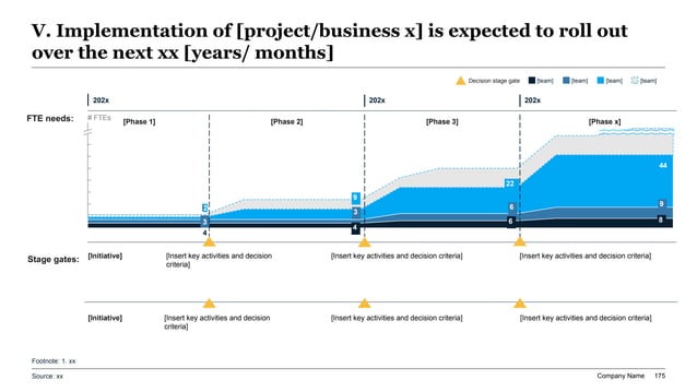
### The 4-Phase Transition Architecture Structure the execution timeline across four sequential phases, as showcased in Exhibit 5:
1. Phase 1: Commercial Alignment, Real Estate RFP & Detailed Engineering (Months 1–6) - Finalize lease negotiations and municipal tax incentive agreements for target sites (Allentown, PA; Dallas, TX; Reno, NV). - Execute detailed facility interior engineering: mezzanine racking layouts, electrical drops, WMS network topology, and MHE equipment procurement. - Issue freight carrier RFPs for realigned lane commitments, locking in dedicated contract rates. - Capital Tranche 1 Release: $8.5M (lease deposits, legal, architectural engineering, and long-lead automation equipment down-payments).
2. Phase 2: Pilot Facility Launch & Parallel Run Testing (Months 7–12) - Complete physical fit-out of primary flagship facility (Allentown Mega-DC). - Install and commission automated sorting systems, conveyor lines, and RF scanning infrastructure. - Execute 60-day end-to-end WMS/ERP parallel testing with mock orders, validating order-to-ship data integrity and barcode scanning accuracy. - Establish temporary 30-day safety stock buffer to ensure zero customer fulfillment disruption during initial warehouse cutover. - Stage-Gate Review 1: Formal presentation to Executive Committee certifying WMS accuracy >= 99.8% and pick-pack-ship throughput testing before authorizing live cutover. - Capital Tranche 2 Release: $24.0M (facility completion, automation installation, inventory stocking).
3. Phase 3: Secondary Regional Node Deployment & Volume Migration (Months 13–18) - Commission remaining regional facilities (Dallas, TX and Reno, NV hubs). - Sequentially migrate regional customer accounts to new shipping nodes in 25% incremental volume waves, monitoring On-Time In-Full (OTIF) delivery metrics daily. - Implement transportation management system (TMS) automated dynamic routing, shifting outbound parcel shipments into optimized local zone bands. - Stage-Gate Review 2: Audit delivered cost-to-serve run-rate against original underwriting assumptions. - Capital Tranche 3 Release: $19.5M (final facility fit-outs and network integration).
4. Phase 4: Legacy Facility Decommissioning, Asset Disposition & Value Realization (Months 19–24) - Complete orderly inventory draw-down at decommissioned legacy warehouses (Memphis, Cleveland, Kansas City, Baltimore). - Terminate legacy warehouse leases or execute industrial real estate sale-leaseback transactions, returning capital to corporate balance sheet. - Settle transition service agreements (TSAs) and reassign local supervisory personnel. - Final Board Governance Review: Present audited 12-month post-transformation P&L statement verifying full $25.7M annual operating savings and $34M inventory reduction.
Exhibit 5: 24-Month Network Migration Roadmap: Phased Transition, Facility Cutovers, and Stage-Gate Capital Tranches
Production-Ready AI Prompt Recipe: Structuring an Institutional Supply Chain Network Optimization Deck in XLSlides
Act as a Senior Operations Strategy Partner at McKinsey & Company and Chief Supply Chain Officer (CSCO) advisor. Structure an executive-ready, 12-slide Supply Chain Network Optimization presentation deck for our Executive Committee and Board of Directors. The business is a $1.2B industrial distributor currently operating 18 fragmented regional warehouses with $142.5M in annual delivered logistics spend, 48% 1-day ground customer reach, and declining operating margins due to freight inflation and redundant inventory holding. We have modeled an optimized 5-node regional distribution network (Allentown PA, Atlanta GA, Indianapolis IN, Dallas TX, Reno NV) that reduces delivered costs by $25.7M annually, slashes safety stock by $34M, and elevates 1-day ground reach to 88.4%. Structure the 12-slide presentation deck strictly following consultant-grade answer-first logic and MECE narrative architecture: - Slide 1: Executive Title Slide & Transformation Thesis with institutional confidentiality disclaimers. - Slide 2: Executive Summary & Capital Allocation Recommendation (The 4 core transformation pillars: Margin Expansion, Working Capital Cash Liberation, Delivery Speed, and Risk Hedging). - Slide 3: Baseline Network Diagnostics (Current 18-facility topology map, cross-shipping inefficiencies, and $142.5M cost-to-serve baseline). - Slide 4: Center-of-Gravity (COG) Demand Centroid Analysis (Visualizing unconstrained mathematical demand centers vs. historical facility drift). - Slide 5: Delivered Cost-to-Serve Optimization Waterfall ($7.83/unit baseline reconciled to $6.45/unit optimized across Inbound Freight, Manufacturing Conversion, Warehousing, and Outbound LTL/Parcel). - Slide 6: Multi-Scenario Network Topology Evaluation Matrix (Side-by-side comparison of Baseline vs. 3-Node Mega-Hubs vs. 16-Node Agile Hub-and-Spoke vs. Recommended 5-Node Regional Hybrid across 9 financial and operational dimensions). - Slide 7: The Supply Chain Trilemma: Service Level (SLA) vs. Outbound Transportation vs. Inventory Working Capital Frontier (Proving the Square Root Law inventory savings). - Slide 8: Multi-Criteria Industrial Real Estate & 3PL Site Selection Scorecard (100-point evaluation across highway connectivity, labor wage density, warehouse clear heights, and tax abatements). - Slide 9: Dedicated Company-Operated vs. Contract 3PL Operating Model Decision Framework (P&L unit cost vs. balance sheet flexibility). - Slide 10: Scope 3 Transportation Decarbonization & Modal Shift Impact (18% CO2 emissions reduction via rail intermodal and localized drayage). - Slide 11: 24-Month Phased Network Transition Roadmap & Stage-Gate Capital Governance (4-phase execution sequence, 3 capital tranches totaling $52M, and customer SLA protection protocols). - Slide 12: Board Resolution & Capital Approval Request (Formal resolution requesting authorization of $52M CapEx and formation of the Supply Chain Transformation Office). For every slide, write a definitive executive Action Title (not a topic title), a crisp 2-sentence executive takeaway banner, detailed quantitative tables with realistic operational parameters, and explicit callout notes for C-suite decision-makers. Ensure no generic marketing fluff.
Common Pitfalls & Anti-Patterns in Supply Chain Executive Presentations
Even quantitatively sound supply chain network studies can fail in the boardroom if the presentation falls into classic operations anti-patterns. Review your deck against these five critical pitfalls before meeting with senior leadership:
1. The 'Spaghetti Map' Visual Trap: - Anti-Pattern: Displaying a raw GIS export showing thousands of individual shipment line traces crisscrossing the country in a chaotic web of overlapping lines. - Executive Impact: Directors cannot discern patterns or insights; the slide looks messy, overwhelming, and unmanaged. - Best Practice: Aggregate freight flows into bold directional corridor bands proportional to annual tonnage. Clearly differentiate primary plant-to-hub linehaul corridors from secondary regional distribution radii using contrasting corporate color codes.
2. Over-Optimizing for Theoretical Lowest Cost while Ignoring Operational Friction: - Anti-Pattern: Selecting warehouse locations based purely on the mathematical lowest-cost coordinate point, even if that coordinate falls in an area with zero industrial warehousing availability, poor truck highway access, or hostile labor union dynamics. - Executive Impact: The board will immediately dismiss the analysis as an academic exercise detached from commercial reality. - Best Practice: Ground mathematical models in real-world feasibility. Clearly document the transition from the theoretical Center-of-Gravity point to real-world sub-market candidate sites that offer shovel-ready industrial parks, 36-foot clear heights, and robust utility power grids.
3. Underestimating Facility Cutover & Parallel-Run OpEx: - Anti-Pattern: Modeling capital expenditures for new buildings while assuming legacy warehouses close instantly on Day 1 without overlapping lease liabilities or redundant inventory buffers. - Executive Impact: CFO scrutiny will expose unbudgeted transition operating costs, destroying project credibility. - Best Practice: Transparently model 60 to 90 days of parallel operating run costs (paying dual rent and temporary supervisory overhead during transition) and allocate a dedicated $3M to $5M operational contingency reserve within the financial model.
4. Presenting Freight Mode Reductions without Carrier Capacity Validation: - Anti-Pattern: Assuming all long-haul trucking volume can instantly shift to rail intermodal to save 22% in transportation costs without verifying rail ramp slot availability or customer lead-time tolerance. - Executive Impact: Supply chain disruptions occur immediately post-launch as rail transit delays trigger customer stockouts and emergency air-freight expedites. - Best Practice: Pair transportation savings models with carrier market capacity testing and contractual commitments from tier-1 freight brokers and intermodal logistics providers.
5. Burying Customer Service Level (OTIF) Impacts: - Anti-Pattern: Focusing 90% of presentation time on internal cost savings while failing to clearly articulate what happens to customer delivery lead times. - Executive Impact: The Chief Commercial Officer (CCO) and sales leadership will oppose the initiative, fearing customer churn and lost market share. - Best Practice: Lead with customer value. Emphasize that the optimized network increases 1-day ground reach from 48% to 88%, positioning sales teams to win enterprise accounts through faster, more reliable delivery.
Frequently Asked Questions About Supply Chain Network Optimization Presentations
How long does an institutional supply chain network optimization study take to complete before presenting to the board?
A comprehensive supply chain network design study typically requires 12 to 16 weeks from project charter to board presentation. Weeks 1–4 focus on data gathering, transaction geocoding, tariff baseline normalization, and capacity constraint audits. Weeks 5–9 involve mathematical modeling, center-of-gravity iterations, and multi-scenario MILP solver runs. Weeks 10–13 focus on industrial real estate due diligence, 3PL market testing, and cost-to-serve waterfall financial reconciliation. Weeks 14–16 are dedicated to executive stakeholder alignment (pre-wiring the CFO, COO, CCO, and CEO) and final board slide deck synthesis.
What is the typical capital expenditure (CapEx) payback period for a regional distribution center consolidation program?
In well-engineered supply chain network transformations, the capital expenditure payback period typically ranges between 1.8 and 3.2 years, with an Internal Rate of Return (IRR) between 25% and 40%. Furthermore, because consolidating facilities releases substantial safety stock inventory (under the Square Root Law), the liberated working capital cash flow often funds between 40% and 70% of total upfront facility fit-out and automation CapEx within the first 12 months.
How should supply chain leaders present geopolitical, tariff, and nearshoring risks to the board?
Present geopolitical and tariff exposure using a scenario-based 'Landed Cost Parity' framework. Contrast total landed costs across three operating theaters: Offshore (e.g., East Asia baseline with maritime freight and Section 301 tariffs), Nearshore (e.g., Mexico under USMCA duty-free rules with 4-day cross-border trucking), and Onshore (domestic US manufacturing). Highlight lead-time volatility, pipeline inventory carrying costs, and currency risk alongside direct wage differentials to prove that nearshoring delivers superior risk-adjusted margins even if direct factory labor rates are marginally higher than offshore alternatives.
What is the difference between greenfield network optimization and brownfield network rationalization?
Greenfield optimization assumes an unconstrained clean-slate environment where the solver identifies the mathematically ideal facility locations without regard to existing corporate assets or historical leases. It serves as an essential theoretical benchmark. Brownfield rationalization, by contrast, takes the existing physical footprint as an active operational constraint—incorporating unexpired lease terms, existing workforce agreements, specialized capital equipment, and customer contracts—and determines the optimal sequence of facility expansions, retrofits, consolidations, and strategic closures.
How do you prevent customer fulfillment disruptions during physical warehouse cutovers?
Operational continuity is maintained through three non-negotiable governance protocols: (1) Running a mandatory 60-day parallel WMS test with zero live customer traffic to validate ERP transaction integrity; (2) Injecting a temporary 30-day safety stock buffer at legacy facilities before cutting over shipping lanes; and (3) Phasing cutovers by customer region or product category in 25% increments rather than executing a high-risk 'Big Bang' transition.
How does supply chain network optimization impact corporate ESG and Scope 3 carbon emissions reporting?
Transportation and warehousing account for the vast majority of Scope 1 and Scope 3 supply chain greenhouse gas emissions. Network optimization directly curtails carbon emissions through three structural mechanisms: (1) Slashing total ton-kilometers traveled by placing distribution hubs closer to customer demand epicenters; (2) Facilitating modal shifts from long-haul diesel trucking to energy-efficient rail intermodal freight (which reduces emissions by up to 65% per ton-mile); and (3) Consolidating into modern LEED-certified, highly insulated distribution centers with rooftop solar installations and automated smart LED energy management.
Why do management consultants recommend pre-wiring executive committee members before the formal presentation?
Supply chain network decisions impact every major corporate stakeholder: the CFO cares about CapEx and working capital; the COO cares about operational throughput; the CCO cares about customer delivery SLAs; and the CHRO cares about workforce relocations and plant severance. Walking into a board meeting without prior alignment invites conflicting executive agendas that derail the project. Pre-wiring involves conducting private 30-minute working sessions with each executive 2 to 3 weeks prior to the board meeting to review their specific functional concerns, incorporate their feedback, and secure individual buy-in.
Transform Complex Supply Chain Network Models into Executive-Ready Decks with XLSlides
Stop wrestling with messy GIS screenshots, dense solver logs, and unreadable spreadsheets. XLSlides empowers operations leaders, supply chain executives, and management consultants to instantly generate institutional, editable PowerPoint slide decks featuring clean center-of-gravity maps, cost-to-serve waterfalls, site selection scorecards, and multi-year transition roadmaps.
Methodology And Sources
- Gartner Magic Quadrant for Supply Chain Network Design Software & Strategy Methodologies(Gartner Research • 2024)
Authoritative industry benchmarking evaluating mixed-integer linear programming (MILP), digital twins, and algorithmic network optimization frameworks.
- Annual State of Logistics Report: Resilience, Capacity Realignment, and Supply Chain Footprint(Council of Supply Chain Management Professionals (CSCMP) & Kearney • 2024)
Foundational empirical research on macroeconomic freight logistics spending, multi-modal linehaul rate benchmarks, and warehouse inventory carrying costs.
- Supply Chain Network Design Under Uncertainty: Balancing Cost, Service, and Disruptive Risk(MIT Center for Transportation & Logistics (CTL) • 2023)
Academic research on center-of-gravity modeling, nearshoring optimization, and stochastic resilience against black-swan supply disruptions.
- Building Resilient Supply Chains: Managing the Trade-Off Between Footprint Cost and Service Velocity(McKinsey & Company Operations Practice • 2024)
Strategic management insights on total landed cost-to-serve decomposition, manufacturing footprint rationalization, and C-suite operational decision-making.
- The New Rules of Supply Chain Strategy: Navigating Nearshoring, Geopolitical Risk, and Cost-to-Serve Optimization(Harvard Business Review • 2023)
Executive framework analyzing the structural shift from single-source offshore manufacturing toward regional, multi-node resilient supply chain architectures.