 XLSlides
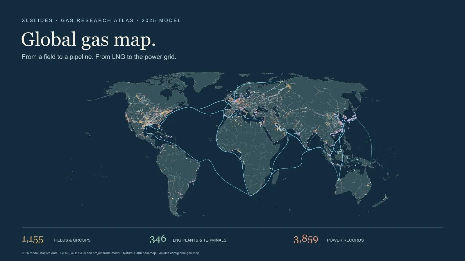
Follow two routes to market
Natural gas reaches a user through infrastructure as well as through a commercial agreement. A producing field may feed a domestic transmission grid, an international pipeline or a liquefaction plant. Gas shipped as LNG passes through additional stages: liquefaction, a sea voyage, receiving-terminal storage and regasification. After delivery it can enter a pipeline network and supply power generation, industrial processes or other demand. A map becomes useful when it separates those stages rather than treating every line as the same kind of connection.
This atlas links the documentary project's gas-field, pipeline, LNG and power-plant records in a single explorable view. Start with a named asset, inspect the record and turn off layers that do not answer your question. A broad geographic view helps establish context. A selected record helps explain the asset definition, reference period, owner and source. Neither view by itself proves that a particular field physically supplied a particular power station.
The reference model is 2025. XLSlides imported the owner's gas project on 30 October 2026, retaining its numerical map values and adding explanatory context. Underlying inventories have different release dates, while individual research inputs can be older. This is a static research snapshot. It does not show current vessel positions, nominations, outages, available capacity or real-time gas prices.
Read the layers in their own units
Gas fields and field groups are circles, with different colours for onshore and offshore records. The production quantity is expressed in billion cubic metres for the reference year. Some records represent an individual field; others represent a basin, play, grouped assets or a residual national allocation. A point is therefore not necessarily a wellhead or a complete outline of an extraction area. The selected panel retains the source input year, source basis, confidence and modelling notes where they can be matched to the project catalogue.
Transmission pipelines are lines that connect locations or networks. Capacity is a potential annual rate, expressed in bcm per year. Flow is the quantity assigned to the reference period. A line with a large capacity can have a much smaller assigned flow, and a record without throughput is not evidence of zero use. The snapshot includes several project statuses. Always inspect status before treating a route as operating infrastructure. Some geometry-backed records have less operating detail than the curated pipeline table.
LNG export plants and import terminals are triangles. The export side turns gas into LNG; the receiving side regasifies imported LNG so it can enter a gas network. The source model distinguishes annual output or imports, in million tonnes, from nameplate capacity, in million tonnes per annum. Capacity and activity should not be substituted for one another. Terminal ownership, an operator, a supplier list and an offtaker relationship can also describe different commercial roles.
LNG lanes are modelled corridors between trading countries. Their curves explain the route and distance assumptions behind a trade relationship. They are not AIS tracks, ship schedules, individual cargoes or a guarantee that every shipment used the illustrated path. An importer can receive LNG from several exporters, and an exporter can supply several markets. The same national trade relationship may also be served through multiple terminals.
Gas-fired power records are squares. The main quantity is nameplate electrical capacity, in MW, rather than gas production or annual generation. The imported snapshot does not have populated 2025 generation figures for these mapped plant records. A blank TWh field means unavailable. It does not mean the plant produced no electricity, nor does it justify estimating a capacity factor without additional evidence. Technology, start-year and site-group notes help distinguish records that may belong to the same wider complex.
Choose a starting point
An upstream starting point is a field or field group such as North Field. Read reference production alongside the source year, national calibration factor and basis notes. A field can have an older input year while its output has been allocated to a 2025 national target. That is different from a direct measurement of the field's 2025 production. For a presentation centred on one field, follow the primary operator or regulator record before relying on the exact quantity.
For an LNG question, try Sabine Pass and inspect the difference between output, capacity and modelled liquefaction fees. Then select a country-to-country corridor such as Qatar to China. The map lets you compare the physical roles of the plant, lane and receiving infrastructure. It does not establish the detailed terms of a sale, the allocation of every train or the identity of every buyer. Those questions need the corresponding contracts, operational disclosures or trade records.
For a demand-side question, try a named gas power plant such as Datan. The plant's MW rating provides a scale reference, while the technology and supply notes identify questions worth researching. A capacity figure alone cannot establish gas consumption. You would also need the operating period, generated electricity, heat rate, fuel mix and other relevant conditions. Keep the plant's capacity comparison separate from a gas-flow comparison unless those extra assumptions are explicit.
Understand country calibration
The original gas project retains a pre-calibration field quantity and a final gas quantity. Its build process scales field allocations to a country target where one is available, then rounds the results. The page's regional and country comparisons use the final calibrated gas column. They do not accidentally sum the similarly named pre-calibration column. This matters because those totals describe different stages of the model.
The inherited labels reported, secondary and modelled describe the project's input provenance. Reported refers to an input attributed to an operator, regulator or government source. Secondary identifies an intermediary account. Modelled identifies an estimated allocation or split. A reported input that is subsequently scaled is no longer an unaltered reported quantity. The selected field therefore shows both its source label and the country's scaling factor where available.
The basis audit counts records. Its modelled percentage is not a percentage of total gas, revenue, countries or geographic accuracy. A small residual group and a large producing field each contribute one record to that count. Confidence labels also come from the source project. XLSlides has not independently reverified every asset, source-year label, ownership record or confidence judgement in this imported snapshot.
Keep volume, energy and electricity apart
bcm means billion cubic metres of gas. A pipeline's capacity may be stated in bcm per year, while a field's reference output is a volume over the model period. Mt means million tonnes of LNG, and Mtpa expresses an annual capacity in million tonnes per annum. Moving between gas volume and LNG mass requires an explicit conversion assumption. Composition, measurement conditions and the definition of the series affect comparisons.
The inherited model uses 1.36 bcm per million tonnes for the gas-equivalent quantity attached to its LNG lanes. That is a project convention for this snapshot, not a universal conversion factor for every cargo. A presentation that relies on a precise conversion should state the convention and check the relevant reporting basis. Do not mix a gas-equivalent volume with a separately reported LNG mass as though they were independent quantities.
MW measures electrical power capacity; TWh measures electrical energy over a period. Neither is interchangeable with a gas volume. MMBtu is an energy unit used in the revenue and tariff assumptions. Heat content is needed when converting between gas volume, LNG mass and energy. A clear exhibit puts the unit and period next to each number rather than leaving the reader to infer them from the map symbol.
Interpret money as a model
The revenue layer uses gas quantities, energy conversions and price assumptions to estimate values at different stages. It includes country and regional price assumptions, pipeline tariffs, liquefaction charges, shipping costs and regasification fees. The project's price file and revenue parameters belong to the captured model. They are not today's tradable prices, quotations for a new contract or audited results for each asset.
Cargo value, liquefaction fees, shipping income and regasification income describe different parts of a chain. They should not be added to claim unique industry revenue without considering repeated valuation of the same gas. A producer's netback also differs from the price paid at the destination. Some owners, traders and offtakers participate in more than one stage, so a physical asset allocation should not be presented as consolidated corporate accounting revenue.
For an illustrative scenario, keep volume, energy content, utilisation, tariff or price, and period in separate cells. Show which assumptions are supplied by the atlas and which you changed for the scenario. If a conclusion depends on one sensitive assumption, make that sensitivity visible. A detailed-looking map is a starting point for this analysis, not a substitute for validating the decisive inputs.
Turn the map into a useful exhibit
Start with a specific question: which supply path matters, which asset is being compared, or what additional infrastructure would a scenario require? Choose the few layers that answer it. A map of every visible record can be useful for orientation, but a decision page usually needs a smaller geographic view and a clearly stated conclusion. Distinguish a documented link from a modelled connection and retain the snapshot date beside the exhibit.
Use an asset table to make the assumptions easy to inspect. For a pipeline, compare capacity, assigned flow and status. For an LNG terminal, compare capacity with the reference output or import volume. For a power plant, show MW and explicitly mark unavailable generation information. The full explorer provides searchable, sortable tables that help find the relevant records, while the JSON download preserves the rendered atlas and its provenance notes.
The companion global oil map provides a useful comparison with a different physical value chain. Our consulting presentation guide explains how to connect action titles, evidence and a recommendation. For a separate scenario, the business-case calculator can help organise assumptions. Keep the analytical scenario separate from what the imported research actually reports.
Coverage and reconciliation remain visible
The merged source catalogue and the rendered map are different populations. The field catalogue contains zero-output records that are not in the production view. The pipeline map contains additional geometry-backed records beyond the curated pipeline table. Power-plant records may represent units or grouped sites. These counts should not be used as competing estimates of the same asset universe.
The source merge report flags country-balance gaps, unresolved destination labels and LNG-terminal allocations that required normalisation. It reports fifteen country balances exceeding both three bcm and ten percent, and eleven flows to unresolved country labels. The page preserves those limitations. A country balance can be affected by storage, statistical definitions, incomplete trade coverage and model assumptions; a gap is not automatically evidence of physical losses.
Use the atlas to discover assets, understand the chain and identify the next source to examine. Before a contractual, operational or investment decision depends on a number, check the operator, regulator, publisher and period that support it. The strongest use of this resource is to make questions and assumptions easier to inspect, rather than to imply certainty that the underlying model does not provide.