 XLSlides
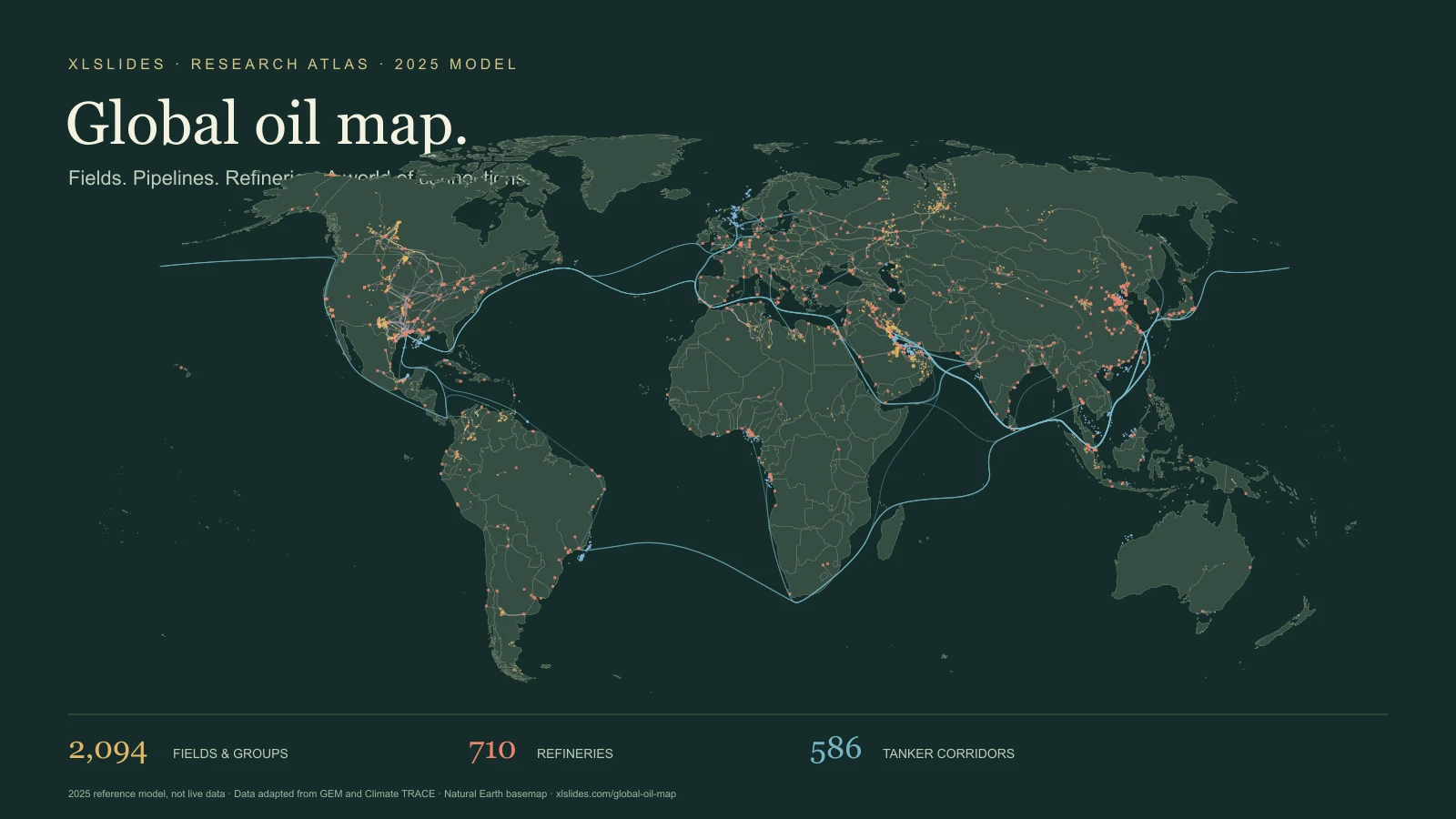
Read the chain, not just the dots
A useful crude-oil map connects production with the infrastructure that turns it into a saleable product. A field shows where liquids enter the system. A gathering network, trunk pipeline or export terminal provides a route to market. A tanker moves cargo between ports. A refinery converts a mixture of crude feedstocks into products with different uses and prices. A country may appear in several of those roles at once.
This atlas brings those layers together so you can examine the relationships. Start with a producing region, find a named asset and inspect its operator, owners and reference output. Then switch on the transport layers and look for the refineries and terminals around it. The result is a research starting point for understanding the value chain, rather than a claim that every visible line proves a particular commercial contract.
The map uses a 2025 reference model assembled for the original documentary project and imported into XLSlides on 29 October 2026. The base inventories come from different releases, and the project adds regional research, estimated allocations and linked flows. It is a reproducible snapshot. It does not update when a tanker moves, a pipeline shuts down or an ownership transaction closes.
What each layer tells you
Oil fields and field groups. Circles represent producing fields or grouped assets, with separate colours for onshore and offshore records. Their size relates to the reference liquids output in the model. Some records aggregate a basin, play or collection of smaller fields. A point should therefore be read as a geographic representation of an asset or group, not as the precise location of every producing well. Search results and the selected record provide more context than the symbol alone.
Pipelines. Lines use the project's pipeline geometry and curated infrastructure records. A line may carry crude, petroleum products or natural gas liquids; the selected record distinguishes the commodity where available. Capacity describes a potential rate of movement, while throughput describes the rate used in the reference model. Those values answer different questions. Construction, idle and operating records can be present, so inspect status before interpreting a route as available transport.
Terminals. Triangles identify export, import or combined terminals. The selected record can show an operator, handling volume and the project's description of incoming supply or main destinations. A terminal's volume is not an additional source of global production. The same oil may be counted first at a field, then at a terminal and again at a refinery as it passes through the chain.
Refineries. Squares represent the mapped refinery inventory. The panel distinguishes nameplate capacity from modelled runs and shows ownership, crude-source notes and product breakdowns where available. A large refinery is not automatically running at full capacity. Product slates and destination channels are also models unless a record explicitly identifies reported output. They are useful for discussing the shape of a business, but do not establish an individual buyer's purchases.
Tanker lanes. Blue corridors represent routed country-to-country trade relationships in the model. They are not AIS tracks, individual voyages or a list of ships currently at sea. Several cargoes and ports can be represented by one corridor. The route helps explain the geographic connection and distance assumption; it does not guarantee that every cargo took the exact curve drawn on the screen.
Three ways to explore
For an upstream question, search for a named field or operator and read the output, ownership and basis together. A number labelled reported has a different evidentiary role from a modelled split of a national total. Use the regional filter to reduce visual density, then compare neighbouring records. If a chart will depend on the exact number, follow the record's source and confirm its year, definition and asset boundary.
For a transport question, begin with the endpoints. A pipeline's capacity, a terminal's handling volume and a tanker lane's trade volume should not be combined without checking whether they describe successive steps in the same journey. Turn layers off to isolate the geography. The atlas can reveal a plausible chain and help you formulate a research question; an assertion about actual contracted flows needs the corresponding primary evidence.
For a downstream question, try a refinery such as Jamnagar and examine the difference between capacity, runs, product sales and gross margin. The product mix indicates the model's allocation of output, while the delivery-channel mix represents an additional set of assumptions. Neither should be treated as audited segment reporting. A presentation should keep the physical activity, the price assumptions and the resulting financial estimate in separate exhibits.
Reported, secondary and modelled are different
The merged field catalogue records three bases. Reported identifies a figure the project attributes to an operator, regulator or government source. Secondary identifies a figure drawn from reporting or an intermediary source. Modelled identifies an allocation or estimate assembled by the project. These are provenance labels carried from the source project. XLSlides has not independently reverified every underlying record.
Most field records and nearly all site-to-site flow records in this snapshot are modelled. The percentages shown in the coverage section are shares of records, not shares of barrels, revenue or geographic accuracy. A small field and a large field each count as one record in that calculation. A model can reconcile to a country's target total while remaining uncertain about the split between individual fields.
Confidence labels add context but do not turn an estimate into a measurement. Some layers lack a confidence or basis field entirely. An empty field means the information is unavailable in this view. It should not be read as zero, no risk, no owner or no activity. When evidence is incomplete, use the atlas to identify what needs checking before making a more precise claim.
Keep barrels, capacity and money separate
The map uses kb/d for thousand barrels per day and mb/d for million barrels per day. A flow of 100 kb/d is 100,000 barrels per day, or 36.5 million barrels over a 365-day year if the rate is constant. The conversion is arithmetic; it does not establish that the asset operated at that rate throughout the year. Crude plus condensate is also a different product boundary from all petroleum liquids or barrels of oil equivalent.
The revenue layer is an illustrative model. Its field calculation starts with output, annualises it over 365 days and applies a Brent assumption of $69 per barrel plus a country differential. That $69 input is an assumption inherited from the project, not a fresh claim about the verified 2025 annual average. Tariffs, terminal fees, freight rates, utilisation and refining margins introduce further assumptions. They should be tested before using the results in an investment or operating decision.
Do not add upstream crude sales, transport income and refined-product sales to claim a unique total market value. The same physical oil is sold and serviced at successive stages. Company ownership allocations also differ from consolidated accounting revenue, and gross margin differs from net profit or cash flow. A good financial presentation states the layer, quantity, period, price basis and exclusions beside the estimate.
From a map to a decision-ready presentation
Begin with a question that has a defined scope: which assets are relevant, which period matters and which physical or financial quantity must be compared? Select the records that answer that question rather than showing every layer at once. A geographic overview can establish context, a small comparison table can expose the assumptions, and a sourced chart can explain the conclusion.
For example, an illustrative supply-chain review might compare a producing field, an export terminal and a refinery. Give each its own row, list the capacity or output definition and distinguish the reported and modelled inputs. Explain which connections are documented and which are the atlas's proposed allocation. A convincing map should make those differences easier to see, rather than hiding them behind visual polish.
Use clear action titles and sourced exhibits when turning the research into a deck. The business-case calculator can help structure a separate scenario, while The Consulting Files explores how incentives, weak evidence and missing challenge can distort a recommendation. Keep the source note, reference period and modelling assumptions visible when exporting a map or chart.
Coverage has boundaries
The catalogue and the rendered map intentionally have different counts. The field catalogue includes zero-output records that are omitted from the production view. The refinery catalogue includes closed and other statuses, while the mapped operational subset is smaller. The pipeline renderer combines curated entries with additional geometry-backed records, so its count exceeds the curated pipeline table. These are different populations, not competing estimates of one total.
There are also known reconciliation gaps. The imported merge report flags two field-flow balances and twenty refinery supply/run balances outside a five-percent tolerance. Three lanes in the revenue model lack usable route paths and are absent from the rendered map. The page retains these limitations instead of silently making the totals agree. They matter if you are trying to reconstruct a specific chain from the model.
Geographic placement and route shape have their own limits. A field may be represented by a centroid, and a modelled sea lane is a simplified corridor. Political boundaries on the basemap are cartographic context. Before using any location, owner or capacity in a contractual or operational setting, consult the relevant operator, regulator or infrastructure record. The atlas is most useful as an explorable research layer with visible provenance.