 XLSlides
Start with a question and an asset
A coal map becomes useful when a geographical observation leads to an inspectable question. A mine can sit close to a railway without using that railway for every delivery. A power plant can share an owner with a mine without consuming all of its production. A port can handle several grades and commodities. Begin with a specific asset, read the selected record and identify what the map actually establishes before drawing a wider conclusion.
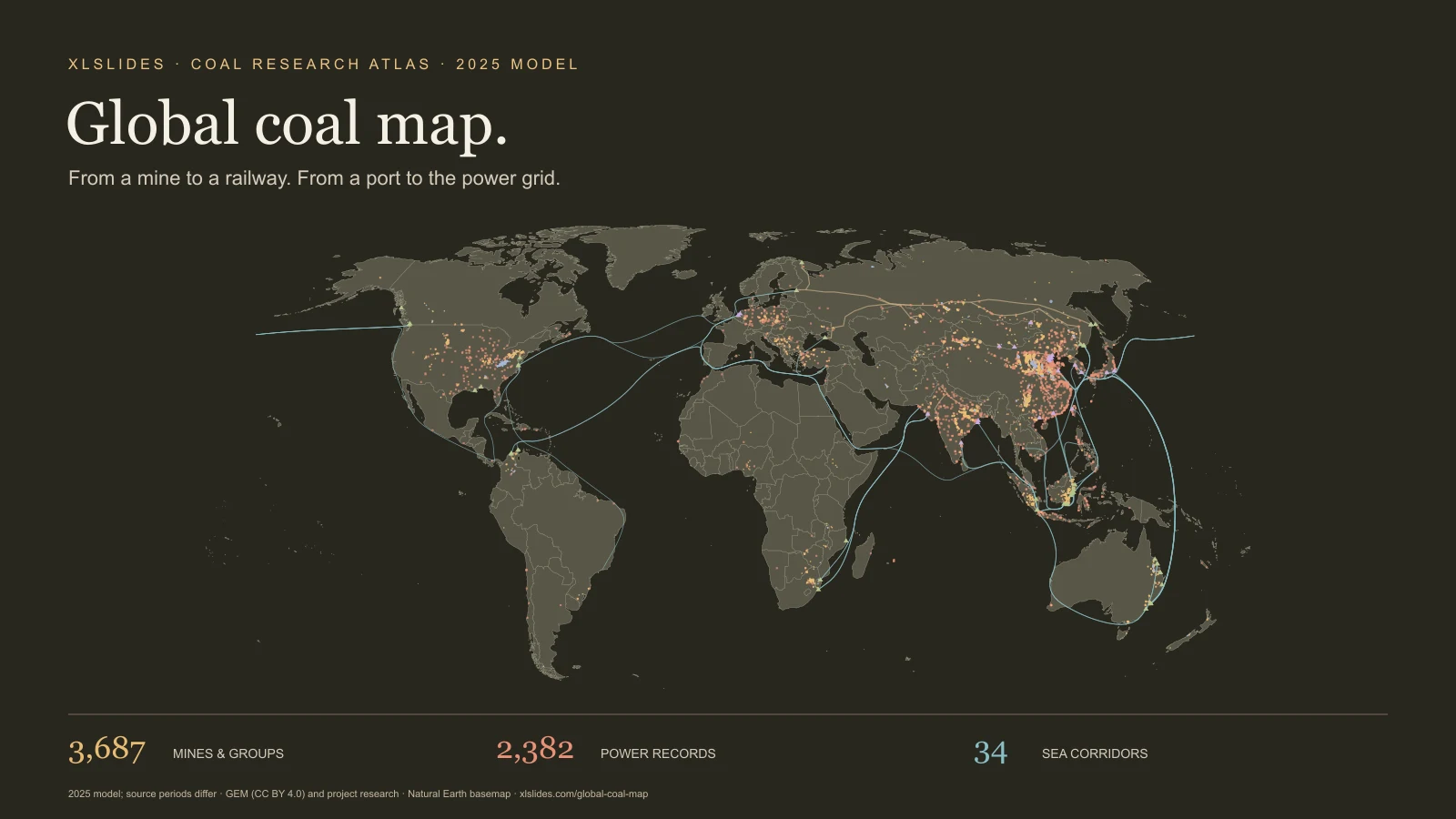
The atlas combines the owner's documentary research on mines, coal-fired power plants, rail corridors, ports and international sea routes. Search for a mine, operator, plant or route; select a result; then reduce the visible layers to those relevant to your question. The full explorer adds searchable and sortable tables. The landing page provides coverage counts and an explanation of the model so the visual can be read alongside its evidence.
The reference model is 2025, imported on 1 November 2026. That does not mean every number is a calendar-2025 observation. Some source inputs describe fiscal years, earlier reporting periods or proxies constructed from more than one year. Inventory releases also have their own dates. This page retains those distinctions instead of presenting a live global monitoring system.
Separate tonnes, capacity and energy
Mine output and coal consumption are expressed in million metric tonnes, abbreviated Mt. Capacity is a potential rate of production or handling, commonly expressed as tonnes per year. Actual output or throughput describes activity during a period. A mine's capacity and its reported production therefore answer different questions. The same distinction applies to a railway or a port.
Coal is not a uniform material. Thermal coal, lignite and metallurgical coal have different uses and characteristics. Moisture, ash content, calorific value and processing all affect what a tonne represents. A comparison of physical tonnes is not automatically a comparison of usable energy, electricity output or steelmaking input. A high-tonnage lignite operation can have a different energy profile from a smaller higher-calorific-value coal operation.
The source project uses saleable coal for Australia while most other country allocations use run-of-mine coal. Run-of-mine material and saleable output describe different stages of production. The page's country and regional charts are sums of these retained model quantities. Treat them as an explanation of the project model, with a visible mixed-basis limitation, rather than as a newly harmonised global production dataset.
Electrical capacity is measured in megawatts, MW. Annual electricity generation is measured here in terawatt-hours, TWh. Neither is interchangeable with Mt of coal. Moving from capacity to generation requires operating-time assumptions; moving from generation to coal use requires efficiency and fuel assumptions. Keep those steps explicit whenever you use the atlas in analysis.
Follow the layers through the system
Mines and mine groups appear as circles. The map separates broad thermal/lignite and coking-coal classifications. A point can represent a named mine, a collection of workings or an allocated group. It is not necessarily a mine boundary, a pit outline or a measurement location. The selected panel preserves the input year, source basis, confidence and available modelling notes.
Coal power plants appear as squares. Their records combine asset capacity with generation, coal-use and emissions fields assembled or modelled in the documentary project. The source and burn-basis labels help explain the quantities, but should not be read as a blanket verification of every field in the record. Plant names can also represent sites rather than a single generating unit.
Ports and crossings appear as triangles. Read the record's role, activity period and scope. An export port, import port, domestic facility and border crossing have different functions. Some catalogue aggregates are deliberately excluded from the map to reduce double counting. Annual throughput should not be substituted for nameplate capacity, and an unpopulated activity field does not establish that a site handled no coal.
Railways show selected schematic connections through towns and logistics nodes. The lines communicate a corridor and its role in the model. They are not surveyed track geometry, train schedules or proof of a named shipment. The limited set of railway records should not be interpreted as the entire world railway network serving coal.
Sea lanes connect selected trading origins and destinations. The curves represent the project's routing assumptions and selected trade relationships. They are not observed vessel tracks or the route followed by every cargo. A national relationship can involve multiple ports, counterparties and grades; a representative port is an explanatory device rather than a complete record of those movements.
Keep reporting periods beside the number
The atlas preserves mixed source periods. Many Indian mine records use FY2024-25. Some Pakistan inputs use another fiscal period. Queensland includes a calendar-year proxy based on fiscal-year figures. Earlier mine observations can also be carried into the model when newer mine-level data was unavailable. The selected record's source input year is part of the meaning of the number.
For a presentation, write the period in the chart label or footnote. “Reference model using mixed calendar and fiscal inputs” is more informative than a broad “2025 data” label. If a decision depends on a change between years, return to the underlying publication and construct a consistent time series. This snapshot alone cannot establish a comparable year-on-year growth rate for every asset.
Input years also differ from inventory publication dates. A tracker release can update the status and location of a facility without providing a newly measured annual production figure. An appointment, ownership change or logistics event after the reference period can have its own date. Preserve the source chronology rather than treating the import date as a universal measurement date.
Read plant burn and emissions as a method
The plant catalogue distinguishes reported, derived and modelled burn records. Those categories describe how the project assembled a quantity. Reported data comes from a cited publication; derived data uses a calculation based on other information; modelled data applies assumptions or allocations. The same record can contain fields with different evidential strength.
For plants without suitable observations, the source model uses electrical capacity and country capacity factors, then scales generation allocations to national coal-generation inputs. Coal consumption is calculated using technology and fuel assumptions, including heat rates and calorific values. CO2 is then related to fuel quantities, energy content and emissions factors. These are model relationships, not direct sensor readings at every plant.
The project notes material limitations. Low assumed lignite calorific values can increase estimated tonnage in some countries. Imported-coal plants in India can be assigned a national fuel assumption that overstates their estimated coal tonnes. The source notes no plant-level Chinese observations in this model. These caveats should remain beside any plant ranking or emissions comparison built from the data.
Do not label every plant's CO2 as verified emissions simply because its coal-use basis is reported. Read the selected source and period, identify which variable it supports and label the rest appropriately. A fair comparison may require a smaller set of consistently measured plants rather than a large table mixing observed and modelled values.
Understand reported inputs and allocated residuals
Most mine records in the catalogue are labelled modelled. Other categories include reported, secondary, reported plus residual and modelled from company totals. Those distinctions matter. A company-level total split between mines using capacity weights remains an allocation, even when the starting company total is reported.
A residual can help reconcile a country or province to a target while leaving uncertainty about its asset-level distribution. An allocated quantity should not acquire false precision simply because it is attached to a detailed coordinate. The selected source notes provide context; the coverage section counts the inherited categories without collapsing mixed categories into uniformly reported observations.
These percentages count records. They are not the share of world coal output, energy, revenue or emissions supported by reporting. A large reported mine and a small modelled mine each contribute one record to the count. If you need a volume-weighted evidence assessment, calculate it separately and explain how mixed and residual categories were treated.
Use four starting points to test a story
Start with Gevra to inspect a mine record and its reporting period. The useful question is how its output and capacity relate to the source description, not simply where its dot appears. Follow with Vindhyachal to inspect a power record and compare the units and basis used for capacity, generation, coal consumption and emissions.
Use Haoji railway to see how a logistics corridor is represented. Read its route, throughput and source before treating the line as an available route for a particular mine. Use Indonesia → China to examine a selected sea-trade connection and its representative ports. Keep the distinction between a national trade relationship and an identified physical cargo.
Together, these starting points provide a way to ask better questions across the chain. They do not establish that the selected mine, railway, port and power plant form a single verified supply path. When a commercial argument requires that connection, add delivery, contract, operator or customs evidence appropriate to the claim.
Build a presentation around inspectable evidence
Choose one decision question before exporting a map image: logistics exposure, the geography of a production portfolio, a plant's fuel assumptions or the concentration of selected trade connections. Use the map for location and relationships, then a small comparison table for quantities. Keep the asset definition, unit, reporting period and evidence basis next to the conclusion.
Avoid a crowded slide that asks a reader to infer the whole model. Show the relevant region or selected layer, explain the observation in the headline and retain the source limitation in a legible note. The consulting presentation guide can help structure the argument; the global oil atlas and global gas atlas provide companion views of other energy systems.
Retain attribution when reusing the downloadable snapshot. The JSON contains the rendered atlas and its provenance notes, not every research CSV or every industrial user in the source project. Review publisher terms and verify the inputs central to your conclusion. This page makes the model easier to inspect; the strength of a recommendation still depends on matching the evidence to the question.